Camera intrinsics: Axis skew

The intrinsic parameters of a camera consist of the focal length, pixel dimensions, the principal point (where the optical axis intersects with the image plane) and finally, the subject of this post, the skew between the axes of the image plane. These parameters are collected into a matrix called the calibration matrix $K$. This calibration matrix is a $3 \times 3$ affine transformation between two 2D spaces (two planes) that gives a way to measure the direction of the ray back-projected from an image point.¹

Usually, the skew coefficient is simply represented as a constant like s and details of how it came about are omitted. To understand why this is so, you might want to skip ahead to the section Should you care about axis skew?). This post aims to discuss in detail, the contribution of the axis skew to the calibration matrix of a camera. To keep the post focused, I assume knowledge of how the other parameters are accounted for in the matrix. The discussion takes the form of a formal solution to a problem in the book “Computer Vision, A Modern Approach”, but I hope that it is self-contained enough to be useful without the book too.

Exercise 1.6

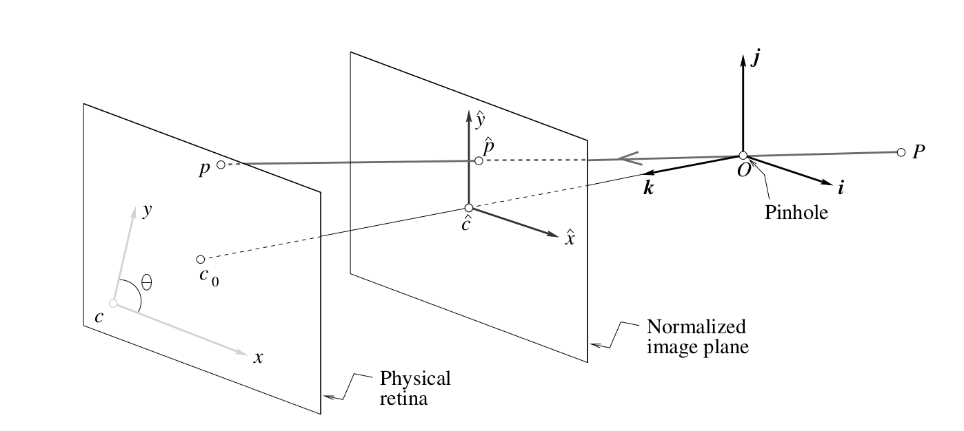
Show that when the camera coordinate system is skewed and the angle $\theta$ between the two image axes is not equal to 90 degrees, then Eq. (1.12) $$x = \alpha\hat{x} + x_0,$$ $$y = \beta\hat{y} + y_0$$

transforms into Eq. (1.13) $$x = \alpha\hat{x} - \alpha cot(\theta)\hat{y}+ x_0,$$ $$y = \dfrac{\beta}{sin(\theta)}\hat{y} + y_0$$

where

• $x$ and $y$ are the pixel coordinates of the projection of a point in the scene onto the retina,
• $\hat{x}$ and $\hat{y}$ are the coordinates of the projection of a point in the scene onto the normalized image plane,
• $\alpha$ and $\beta$ are the pixel magnification factors along the $x$ and $y$ axes respectively,
• and $x_0$ and $y_0$ are the offsets of the image center from the origin of the camera coordinate system ².

Solution Outline

Let the ideally aligned axes of the normalized image plane with zero skew represent the axes of the coordinate frame $Norm$ and the skewed axes represent the axes of the coordinate frame $Skew$.

Note that $Norm$ and $Skew$ share the bottom left corner by construction.

Exercise 1.6 then can be rephrased in the following manner.

Given the pixel coordinates of a point in frame $Norm$, prove that its pixel coordinates in frame $Skew$ is given by Eq. (1.13).

I always find that rephrasing a problem in multiple ways helps clarify the question further. So, yet another way of rephrasing the problem is as follows.

Given the pixel in the normalized image grid that is activated by a perspective ray from a point in the scene, prove that the pixel on the skewed pixel grid that is activated by the same ray is given by Eq. (1.13).

The crux of the solution is that the problem has two parts.

Firstly, a point on the image plane is represented in the camera coordinate system not in the normalized image plane coordinate system. Up until now, we didn’t have to note the difference because both were identical (cartesian). After the skew transformation, the camera coordinate system is different from the normalized image plane coordinate system. So we must learn how to represent a point in the skewed camera coordinate system in terms of its known coordinates in the normalized image plane system.

Secondly, we have not yet defined the relationship between the skewed pixel grid and the normalized image plane grid. How exactly did I generate the picture of the skewed image grid you might ask? Good question. It turns out that there are multiple ways to transform the skewed pixel grid to a normalized grid with axes perpendicular to each other. This took quite some time to sink into my head and would have saved my head and the wall quite a bit of bother if the authors had mentioned upfront which transformation they were using. I say this because almost everyone else (Matlab³, other books^{4 5}) uses a different transform and hence ends up with an equation that is different from Eq. (1.13) and thus a different calibration matrix!

I talk about the transformation from the skewed grid to the normalized grid because the skewed grid is the real image plane/retina whereas the normalized image plane is something we have conjured up to make the math easier. However, as the intrinsic parameters $\alpha$ and $\beta$ are defined with respect to the normalized image plane in the book, we will use the inverse of this transform in our proof. So from now on, we’ll talk about transforming the normalized grid to the skewed grid.

Finally, using the skewed frame coordinates we obtain in the first part together with the pixel dimensions we obtain based on the transformation we chose in the second part, we can find the pixel coordinates on the skewed grid, thus deriving Eq. (1.13).

Solution

1. Finding image coordinates of a point in the skewed frame.

I’m going to do this two ways. The first explanation is more elaborate but requires only basic knowledge of linear algebra and geometry. The second one is more straightforward but requires at least intermediate knowledge of linear algebra.

Using geometry and basic linear algebra

The coordinates of a point in a given coordinate frame is simply a linear combination of the frame axes. This means that the point can be represented as a weighted sum of $n$ axis vectors of the frame. In this case, we only have 2 axes as the point lies on the 2D image plane.

Using the parallelogram law of vector addition, we can geometrically represent the point in both the frames as the diagonal of the parallelogram formed by drawing vectors, parallel to the axes, to the point as shown in the following figures.

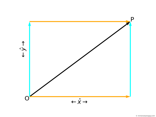
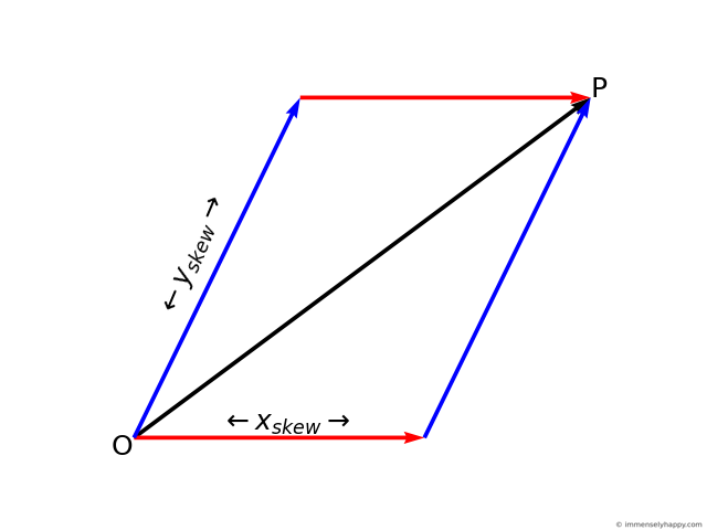
Just as the length of edges of the parallelogram in frame $Norm$, $\hat{x}$ and $\hat{y}$, are the coordinates of point P in frame $Norm$, the length of the edges of the parallelogram in frame $Skew$, $x_{skew}$ and $y_{skew}$, are the coordinates of the point P in frame $Skew$. Another way to think about this is that the length of the edges are the weights in the weighted sum (linear combination) of the axes.

Superimposing both these coordinate frames so that their origins coincide, we can use geometry and trigonometry to find the length of the edges of the parallelogram in frame $Skew$ (in blue and red) in terms of the coordinates of the point in frame $Norm$ (in cyan and orange).

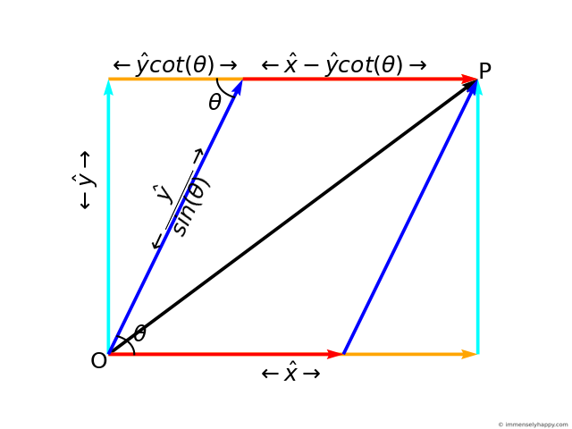
As you can see

$$x_{skew} = \hat{x} - \hat{y}cot(\theta)$$ $$y_{skew} = \dfrac{\hat{y}}{sin(\theta)}$$

Changing the basis

This problem is equivalent to a change of basis problem⁶ with the old basis being the standard basis for $R^2$

$$I = \begin{pmatrix}1 & 0\\ 0 & 1\end{pmatrix}$$

and the new skewed basis being

$$O = \begin{pmatrix}1 & cos(\theta)\\ 0 & sin(\theta)\end{pmatrix}.$$

If the coordinates of a point in the old basis is $\hat{x}, \hat{y}$. The the coordinates of that point in the new basis will be

$$\begin{pmatrix}x_{skew} \\ y_{skew}\end{pmatrix} = O^{-1} I \begin{pmatrix}\hat{x} \\ \hat{y}\end{pmatrix}.$$

$$\implies \begin{pmatrix}x_{skew} \\ y_{skew}\end{pmatrix} = \begin{pmatrix}1 & -cot(\theta)\\ 0 & \frac{1}{sin(\theta)}\end{pmatrix} \begin{pmatrix}\hat{x} \\ \hat{y}\end{pmatrix}.$$

$$\implies \begin{pmatrix}x_{skew} \\ y_{skew}\end{pmatrix} = \begin{pmatrix}\hat{x} - \hat{y}cot(\theta) \\ \frac{\hat{y}}{sin(\theta)}\end{pmatrix}.$$

Just like that! *snaps fingers*.

2. Choosing the appropriate transformation

A hint as to what transform could be in play is in the use of the word “skew” to represent the state of the pixel grid whose axes are not quite perpendicular to each other. Skew is a synonym for shear and we know that the shear transform can be represented as

$$T_{shear} = \begin{pmatrix}1 & cot(\theta)\\ 0 & 1\end{pmatrix}.$$

This is what a sheared grid (in blue) corresponding to the normalized image grid (in black) looks like.

Notice that the blue and black horizontal lines overlap and the height of the pixel (slanted line) in the sheared grid is longer than the height of the pixel (vertical line) in the normalized grid. In fact, $$pixelHeight_{sheared} = \dfrac{pixelHeight_{normalized}}{sin(\theta)}$$ which proves that when $\theta < 90$ $$pixelHeight_{sheared} > pixelHeight_{normalized}$$

Now $$\beta = \dfrac{f}{pixelHeight}.$$ Hence as $f$ (the focal length) and the width of the pixels remain unaffected by the shear transformation, we get $$\beta_{sheared} = \beta_{normalized}sin(\theta) = \beta sin(\theta)$$ $$\alpha_{sheared} = \alpha_{normalized} = \alpha.$$

What if I don’t want the pixel dimensions and hence $\beta$ to change? The following matrix produces a “skew” without changing the dimensions of the pixel. I got this matrix by drawing out the normalized pixel and skewed pixel with the same width and height, then using trigonometry to derive the relationship between their x and y coordinates. $$T_{skew} = \begin{pmatrix}1 & cos(\theta)\\ 0 & sin(\theta)\end{pmatrix}$$

Hence by construction $$\beta_{skewed} = \beta_{normalized} = \beta$$ $$\alpha_{skewed} = \alpha_{normalized} = \alpha.$$

Which is the correct transformation though? For this proof the appropriate transformation is $T_{skew}$, the one that preserves pixel dimensions. However, the answer in general is either/both. The normalized image plane is whatever you make it to be as long as its axes are perpendicular to each other and its left bottom aligns with the actual pixel grid. If you want to use the shear transform you would have to adjust the Eq. (1.13) (as we will discuss later).

3. Finding pixel coordinates of a point in the skewed frame.

Now, as

1. perspective projection proportionality holds even when the $X$ and $Y$ axes are not perpendicular to each other,
2. the pixel dimensions remain unchanged by the chosen skew transformation (as proved in the previous section) and,
3. the focal length ($f$) and distance to object ($Z$) remain unaffected by the skew

Eq. (1.12) also holds for skewed coordinates. Hence

$$x = \alpha x_{skew} + x_0,$$ $$y = \beta y_{skew} + y_0.$$

Replacing $x_{skew}$ and $y_{skew}$ with their values in terms of the normalized image plane coordinates, we get

$$x = \alpha(\hat{x} - \hat{y}cot(\theta)) + x_0,$$ $$y = \beta\dfrac{\hat{y}}{sin(\theta)} + y_0$$

$$\implies$$

$$x = \alpha\hat{x} - \alpha cot(\theta)\hat{y}+ x_0,$$ $$y = \dfrac{\beta}{sin(\theta)}\hat{y} + y_0.$$

where $x$ and $y$ are pixel coordinates of the image point in the skewed coordinate frame. This is the same as Eq. (1.13).

Also, when $\theta = 90$ degrees, $cot(\theta) = 0$, $sin(\theta) = 1$ and the equation reduces to

$$x = \alpha\hat{x} + x_0,$$ $$y = \beta\hat{y} + y_0$$

This proves that Eq. (1.12) transforms into Eq. (1.13) when the angle $\theta$ between the image axes is not 90 degrees.

Pixel coordinates with the shear transform

When we use a shear transform to convert the normalized pixel grid to the skewed one, Eq. (1.13) becomes

$$x = \alpha\hat{x} - \alpha cot(\theta)\hat{y}+ x_0,$$ $$y = \dfrac{\beta_{sheared}}{sin(\theta)}\hat{y} + y_0.$$

Substituting the value of $\beta_{sheared}$ we derived in an earlier section we get

$$y = \dfrac{\beta sin(\theta)}{sin(\theta)}\hat{y} + y_0.$$ $$\implies$$ $$y = \beta\hat{y} + y_0.$$

So the pixel coordinates of a point in the skewed coordinate frame are given by $$x = \alpha\hat{x} - \alpha cot(\theta)\hat{y}+ x_0,$$ $$y = \beta\hat{y} + y_0$$

where $-\alpha cot(\theta)$ is also known as the skew coefficient $s$ in many places. This results in a calibration matrix that has the familiar form that we see in Matlab and other books too.

$$K = \begin{pmatrix}\alpha & s & x_0\\ 0 & \beta & y_0\\0 & 0 & 1\end{pmatrix}.$$

Note that Matlab states the skew parameter as equivalent to $+\alpha cot(\theta)$. This sign change is because the origin is in the top left corner and the $y$ axis increases as we go down⁷.

Should you care about axis skew?

Whew, that was a lot of work! You might be relieved to know that you don’t have to consider the axis skew for most modern cameras because the axes of modern CCD cameras are usually at $90^\circ$ with respect to each other.

Here’s an excerpt from the section “Camera Intrinsics” on page 46 of the book Computer Vision Algorithms and Applications by Richard Szeliski.

Note that we ignore here the possibility of skew between the two axes on the image plane, since solid-state manufacturing techniques render this negligible.

And here are excerpts from the sections “Finite projective camera” and “When is s $\ne$ 0” on pages 143 and 151 respectively of the book Multiple View Geometry in Computer Vision by Richard Hartley and Andrew Zisserman.

The skew parameter will be zero for most normal cameras. However, in certain unusual instances it can take non-zero values.

A true CCD camera has only four internal camera parameters, since generally s = 0. If s $\ne$ 0 then this can be interpreted as a skewing of the pixel elements in the CCD array so that the x- and y- axes are not perpendicular. This is admittedly very unlikely to happen.

In realistic circumstances a non-zero skew might arise as a result of taking an image of an image, for example if a photograph is re-photographed, or a negative is enlarged. Consider enlarging an image taken by a pinhole camera (such as an ordinary film camera) where the axis of the magnifying lens is not perpendicular to the film plane or the enlarged image plane.

In fact, OpenCV⁸ does away with the skew parameter altogether and its calibration matrix looks like

$$K = \begin{pmatrix}\alpha & 0 & x_0\\ 0 & \beta & y_0\\0 & 0 & 1\end{pmatrix}.$$

To sum up, you would need to account for axis skew when calibrating unusual cameras or cameras taking photographs of photographs, else you can happily ignore the skew parameter.

Acknowledgments

Thanks to automoto for your invaluable review.

References

comments powered by Disqus