Multiple View Geometry in Computer Vision Chapter 5 Solutions

Whew! This chapter took much longer to process than I had anticipated. It was mainly because I had to stop every few pages to revisit a concept in linear algebra or probability. So I’m listing out those concepts below in the hope that it will be helpful to anyone attempting this chapter.

1. Vector subspaces (the column space, row space, nullspace and left nullspace), their dimensions, and the orthogonality relationships between them.
2. Expectation and variance of a random variable and the relationship between them (via the second moment).
3. Using Jacobians and first-order approximations.
4. Covariance matrices as a measure of uncertainty.
5. Generalized least squares.
6. Multivariate normal distributions, especially anisotropic ones.

Chapter 12 of the book “Introduction to Linear Algebra” by Gilbert Strang is pretty useful for the last three concepts.

Apart from the exercise solutions, there are some notes/proofs that I would like to provide to clarify some of the matter in the text.

1. Derivation of RMS residual and estimation errors.
   If you’re wondering, like I did, why the expectation of the squared term equals the variance, this is because of the following rule $$Var(X) = E(X^2) - E(X)^2$$ In this case, the error, by assumption, has zero mean. So, $E(\begin{Vmatrix}X - \hat{X}\end{Vmatrix}) = E(\begin{Vmatrix}\bar{X} - \hat{X}\end{Vmatrix}) = 0$. Hence, we get $$\epsilon^2_{res} = E(\begin{Vmatrix}\hat{X} - X\end{Vmatrix}^2/N) = \frac{1}{N}E(\begin{Vmatrix}\hat{X} - X\end{Vmatrix}^2) \\ = \frac{1}{N}Var(\begin{Vmatrix}\hat{X} - X\end{Vmatrix}) = \frac{1}{N}(N - d)\sigma^2$$ where $\epsilon^2_{res}$ is the Mean Square Error or MSE (not root mean square error RMSE). $RMSE = \sqrt{MSE}$.

2. RMS residual and estimation errors for anisotropic error distributions.
   The random variable $\begin{Vmatrix}X - \hat{X}\end{Vmatrix}_\Sigma^2$ has a $\chi^2$ distribution¹ with degrees of freedom equal to the dimension of the underlying normally distributed random variable ($N - d$ in this case). The expectation of a $\chi^2$ random variable is equal to its degrees of freedom. Hence, $$E(\begin{Vmatrix}X - \hat{X}\end{Vmatrix}_\Sigma^2) = N - d$$ $$E(\begin{Vmatrix}\overline{X} - \hat{X}\end{Vmatrix}_\Sigma^2) = d$$ And the respective RMS errors will be $$\epsilon_{res} = \sqrt{1 - d/N}$$ $$\epsilon_{est} = \sqrt{d/N}$$

3. Proof of Result A5.2(p591).
   Honestly, I didn’t understand the argument for sufficiency in the sketch proof so I’ll provide my own. We need to prove that if $N_L(X) = N_L(A)$, then $A^{+X} = X(X^TAX)^{-1}X^T = A^+$.

   • From the definition of $A^{+X}$, we can see that $N_L(X) \subseteq N_L(A^{+X})$ and as we know that the left nullspaces of $X$ and $A^{+X}$ have the same dimension ($M - d$) these two nullspaces must be equal. Furthermore, as $A^{+X}$ is symmetric this is also its right nullspace. Hence $N_L(A^{+X}) = N_R(A^{+X}) = N_L(X)$
   • Now $A^+ = UD^+U^T$ and $A = UDU^T$. As the last $(M - d)$ columns of $U$ contain the basis for the left nullspace of both $A^+$ and $A$, they both must have the same left, and by symmetry right, nullspaces. Hence $N_L(A^+) = N_R(A^+) = N_L(A)$
   • As $N_L(A) = N_L(X)$, we get $N_L(A^{+X}) = N_R(A^{+X}) = N_L(A^+) = N_R(A^+)$.
   • This further implies that the row spaces and column spaces of the two matrices $A^+$ and $A^{+X}$ are equal as they both are $M\times M$ matrices of rank $d < M$.
   • When all four vector subspaces of two singular matrices are the same, they must be the same matrix. Hence $A^{+X} = A^+$ when $N_L(A) = N_L(X)$. Note: This does not apply to invertible matrices.

4. Whenever the authors refer to “noise/error of 1 pixel”, what they actually mean is that the errors come from a multivariate normal distribution with zero mean and a standard deviation of 1 pixel in each coordinate.

The main index for all chapters can be found here.

I. Consider the problem of computing a best line fit to a set of 2D points in the plane using orthogonal regression. Suppose that $N$ points are measured with independent standard deviation of $\sigma$ in each coordinate. What is the expected RMS distance of each point from a fitted line?

The RMS distance of each point from the fitted line is nothing but the RMS residual error of the orthogonal regression estimator.

Following the discussion from Section 4.2.7(p101), we need to define the dimensions of the measurement space and the model to arrive at the answer.

The measurement space clearly consists of all sets of coordinates of $N$ points, N $x$ and N $y$ coordinates, i.e. $\mathbb{R}^{2N}$. The dimension of this space is $2N$.

The model in this case is a subset $S$ of points in $\mathbb{R}^N$ that lie on a line. We only need 2 points to define a line, so the dimension of the model is $2 * 2 = 4$, i.e. a feasible choice of points making up the submanifold $S \subset \mathbb{R}^N$ is determined by a set of 4 parameters, $\hat{x}_1, \hat{y}_1, \hat{x}_2, \hat{y}_2$.

Using these values in conjunction with result 5.1(p136) we get

$$\epsilon_{res} = \sigma(1 - \frac{4}{2N})^\frac{1}{2} = \sigma(\frac{N - 2}{N})^\frac{1}{2}$$

Just to be sure (and to generate pretty graphs), I also verified this result experimentally in Octave.

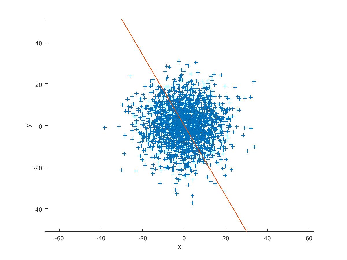
The first graph is just to show you what the best fit line using orthogonal regression would look like for a sample of 2000 points taken from a bivariate normal distribution with zero mean and a standard deviation of 10 in each coordinate.

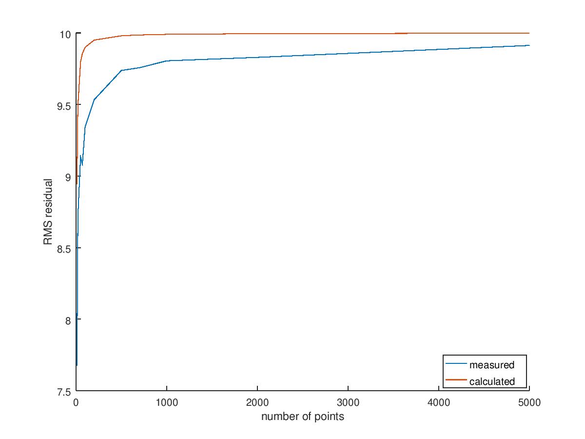
The second graph shows that the estimated value closely tracks the closed form $\epsilon_{res}$ we just calculated and both of them tend to $\sigma = 10$ as the number of points tend to infinity.

If you’re interested in the Octave/Matlab code for this, I’ve uploaded it over here.

II. In section 18.5.2(p450) a method is given for computing a projective reconstruction from a set of $n + 4$ point correspondences across $m$ views, where 4 of the point correspondences are presumed to be known to be from a plane. Suppose the 4 planar correspondences are known exactly, and the other $n$ image points are measured with 1 pixel error (each coordinate in each image). What is the expected residual error of $\begin{Vmatrix}\textbf{x}_j^i - \hat{P^i}\textbf{X}_j\end{Vmatrix}$?

As this is a problem from a much later section, I do not understand it very well yet and will come back to it later (if I remember to).

References

comments powered by Disqus