Multiple View Geometry in Computer Vision Chapter 8 Solutions

Here’s a quick index to all the problems in this chapter.

i ii iv vii viii ix x xi xii xiii xiv xv

The main index can be found here.

I. Homography from a world plane. Suppose $H$ is computed (e.g. from the correspondence between four or more known world points and their images) and $K$ known, then the pose of the camera $\{R, \textbf{t}\}$ may be computed from the camera matrix $[\textbf{r}_1, \textbf{r}_2, \textbf{r}_1 \times \textbf{r}_2, \textbf{t}]$, where $$[\textbf{r}_1, \textbf{r}_2, \textbf{t}] = \pm K^{-1}H/||K^{-1}H||.$$ Note that there is a two-fold ambiguity. This result follows from (8.1-p196) which gives the homography between a world plane and calibrated camera $P = K[R|\textbf{t}]$.
Show that the homography $\textbf{x} = H\tilde{\textbf{X}}$ between points on a world plane $(\textbf{n}^T, d)^T$ and the image may be expressed as $H = K(R - \textbf{tn}^T/d)$. The points on the plane have coordinates $\tilde{\textbf{X}} = (X, Y, Z)^T$

This proof is based on the notes by Marc Pollefeys¹.

A point on the world plane in homogeneous coordinates is $\textbf{X} = (\tilde{\textbf{X}}, 1)^T$. As these points are constrained to lie on the plane $(\textbf{n}^T, d)^T$, they must satisfy

$$(\textbf{n}^T, d)\textbf{X} = 0$$ $$(\textbf{n}^T, d)\begin{pmatrix}\tilde{\textbf{X}} \\ 1\end{pmatrix} = 0$$ $$\implies \textbf{n}^T\tilde{\textbf{X}} + d = 0$$ $$\implies -\frac{\textbf{n}^T\tilde{\textbf{X}}}{d} = 1$$

This means, we can rewrite the homogeneous point $\textbf{X}$ as

$$\begin{pmatrix} \tilde{\textbf{X}} \\ -\frac{\textbf{n}^T\tilde{\textbf{X}}}{d} \end{pmatrix}$$ $$ = \begin{pmatrix} I_{3 \times 3} \\ -\frac{\textbf{n}^T}{d} \end{pmatrix}\tilde{\textbf{X}}$$

Applying the projective transformation $P$ to this point, we get the image as $$\textbf{x} = K[R | \textbf{t}]\begin{pmatrix} I_{3 \times 3} \\ -\frac{\textbf{n}^T}{d} \end{pmatrix}\tilde{\textbf{X}}$$ $$\implies \textbf{x} = K(R - \textbf{tn}^T/d)\tilde{\textbf{X}}$$

Hence, the image of a point on a plane is related it by the homography $H = K(R - \textbf{tn}^T/d)$.

II. Line projection.
(a) Show that any line containing the camera centre lies in the null-space of the map (8.2-p198), i.e. it is projected to the line $\textbf{l} = \textbf{0}$.
(b) Show that the line $\mathcal{L} = \mathcal{P}^T\textbf{x}$ in $\mathbb{P}^3$ is the ray through the image point $\textbf{x}$ and the camera centre. Hint: start from result 3.5(p72), and show that the camera centre $\textbf{C}$ lies on $\mathcal{L}$.
(c) What is the geometric interpretation of the columns of $\mathcal{P}$?

(a) If the line $L$ contains the camera center $C$ then its Plücker matrix is given by $L = AC^T - CA^T$, where $A$ is another point on the line. Substituting this in equation 8.2, we get

$$[\textbf{l}]_{\times} = P(AC^T - CA^T)P^T$$ $$= PAC^TP^T - PCA^TP^T$$ $$= PA(PC)^T - (PC)(PA)^T$$ $$= 0$$

as $C$ is in the nullspace of $P$. Hence, any line containing the camera centre is projected to the line $\textbf{l} = \textbf{0}$

(b) This proof is provided as the proof of proposition 8 in ².

In summary, if we consider the three planes $xP^2 - yP^1$, $xP^3 - wP^1$ and $yP^3 - wP^2$, where $\textbf{x} = (x, y, w)^T$, we can prove (using the dot product of a plane and a point) that each of these planes contains both the centre $C$ and the point $\textbf{X}$. Hence $C$ and $\textbf{X}$ must lie on the line of intersection of these planes. Furthermore, using the definition of Plücker matrices as an intersection of planes, we can prove that this line of the intersection of the three planes is $\mathcal{P}^Tx$. As $\textbf{x}$, by definition, lies on the line between $C$ and $\textbf{X}$, it also lies on $\mathcal{P}^T\textbf{x}$.

(c) The columns of $\mathcal{P}$ are the vanishing lines of the world $x$, $y$, $z$ axes and the $xy$, $yz$ and $zx$ planes. For example the $x$ axis has Plücker coordinates $(0, 0, 1, 0, 0, 0)$, and it is imaged at $\mathcal{P}(0, 0, 1, 0, 0, 0)^T = \mathcal{P}^3$, the $3^{rd}$ column of $\mathcal{P}$.

IV. Apparent contour of an algebraic surface. Show that the apparent contour of a homogeneous algebraic surface of degree $n$ is a curve of degree $n(n - 1)$. For example, if $n = 2$ then the surface is a quadric and the apparent contour a conic. Hint: write the surface as $F(X, Y, Z, W) = 0$, then the tangent plane contains the camera center $C$ if $$C_X\frac{\partial{F}}{\partial{X}} + C_Y\frac{\partial{F}}{\partial{Y}} + C_Z\frac{\partial{F}}{\partial{Z}} + C_W\frac{\partial{F}}{\partial{W}} = 0$$ which is a surface of a degree $n - 1$.

The contour generator will lie³ at the intersection of the tangent surface of degree $n - 1$ and the algebraic surface of degree $n$. By Bezout’s theorem (the degree of a complete intersection of hypersurfaces is the product of the degrees of the hypersurface), we can conclude that the contour generator will have degree $n(n-1)$. Finally, as the algebraic curve is homogeneous, any projective transformation of the contour will also have degree $n(n - 1)$. Hence, the apparent contour will have degree $n(n - 1)$.

VII. Show that the imaged circular points of a perspectively imaged plane may be computed if any of the following are on the plane: (i) a square grid; (ii) two rectangles arranged such that the sides of one rectangle are not parallel to the sides of the other; (iii) two circles of equal radius; (iv) two circles of unequal radius.

If we can find the homography $H$ between the plane and its image with the given information, we can compute the imaged circular points as $H(1, \pm i, 0)$ or $\textbf{h}_1 \pm i\textbf{h}_2$.

(i) The procedure to find the homography is the same as that in step (i) of Example 8.18, A simple calibration device (p211).

(ii) We can use the two step metric rectification procedure in this case

1. Affine rectification: Find two vanishing points using the two sets of parallel lines in one of the rectangles. The join of these points will be the vanishing line. Use this to affine rectify the image using equation 2.19(p49).
2. Metric rectification: Each rectangle gives one orthogonality constraint between a pair of lines. Use this to perform metric rectification as in Example 2.26 (p56).

The composition of these two transformations will give us the projective transformation $H$ that maps the rectangle to the imaged points up to a similarity.

(iii) and (iv) We only need one circle really. We can get 5 orthogonality constraints from an imaged circle using the fact that the inscribed angle of the diameter is $90^{\circ}$. This can be used as in Example 2.27(p 56) to determine the homography $H$.

VIII. Show that in the case of zero skew, $\omega$ is the conic $$\frac{x - x_0}{\alpha_x}^2 + \frac{y - y_0}{\alpha_y}^2 + 1 = 0$$ which may be interpreted as an ellipse aligned with the axes, centred on the principal point, and with axes of length $i\alpha_x$, and $i\alpha_y$ in the $x$ and $y$ directions respectively.

In the case of zero skew, the matrix $K$ will have the form

$$\begin{pmatrix} \alpha_x & 0 & x_0 \\ 0 & \alpha_y & y_0 \\ 0 & 0 & 1 \end{pmatrix}$$

Hence, $\omega = (KK^T)^{-1}$ will be $$\begin{pmatrix} \frac{1}{\alpha_x^2} & 0 & -\frac{x_0}{\alpha_x^2} \\ 0 & \frac{1}{\alpha_y^2} & -\frac{y_0}{\alpha_y^2} \\ -\frac{x_0}{\alpha_x^2} & -\frac{y_0}{\alpha_y^2} & \frac{y_0^2}{\alpha_y^2} + \frac{x_0^2}{\alpha_x^2} + 1 \end{pmatrix}$$

This represents the conic $$\frac{x^2}{\alpha_x^2} - 2\frac{x_0x}{\alpha_x^2} + \frac{x_0^2}{\alpha_x^2} + \frac{y^2}{\alpha_y^2} - 2\frac{y_0y}{\alpha_y^2} + \frac{y_0^2}{\alpha_y^2} + 1 = 0$$

$$= (\frac{x - x_0}{\alpha_x})^2 + (\frac{y - y_0}{\alpha_y})^2 + 1 = 0$$

IX. If the camera calibration $K$ and the vanishing line $\textbf{l}$ of a scene plane are known then the scene plane can be metric rectified by a homography corresponding to a synthetic rotation $H = KRK^{-1}$ that maps $\textbf{l}$ to $\textbf{l}_\infty$, i.e. it is required that $H^{-T}\textbf{l} = (0, 0, 1)^T$. This condition arises because if the plane is rotated such that its vanishing line is $\textbf{l}_\infty$ then it is fronto-parallel. Show that $H^{-T}\textbf{l} = (0, 0, 1)^T$ is equivalent to $R\textbf{n} = (0, 0, 1)^T$, where $\textbf{n} = K^T\textbf{l}$ is the normal to the scene plane. This is the condition that the scene normal is rotated to lie along the camera $Z$ axis. Note the rotation is not uniquely determined since a rotation about the plane’s normal does not affect its metric rectification. However, the last row of $R$ equals $\textbf{n}$, so that $R = [\textbf{r}_1, \textbf{r}_2, \textbf{n}]^T$ where $\textbf{n}$, $\textbf{r}_1$ and $\textbf{r}_2$ are a triad of orthonormal vectors.

Substituting $H = KRK^{-1}$ in the condition that $H^{-T}\textbf{l} = (0, 0, 1)^T$, gives

$$(KRK^{-1})^{-T}\textbf{l} = (0, 0, 1)^T$$ $$\implies (KR^{-1}K^{-1})^{T}\textbf{l} = (0, 0, 1)^T$$ $$\implies (KR^{T}K^{-1})^{T}\textbf{l} = (0, 0, 1)^T$$ $$\implies (K^{-T}RK^T)\textbf{l} = (0, 0, 1)^T$$ $$\implies (K^{-T}RK^T)K^{-T}\textbf{n} = (0, 0, 1)^T$$ $$\implies K^{-T}R\textbf{n} = (0, 0, 1)^T$$

Multiplying both sides by $K^T$, we get $$R\textbf{n} = K^T(0, 0, 1)^T$$

$K^T(0, 0, 1)^T$ will be equal to the last column of $K^T$ or the last row of $K$ which is $(0, 0, 1)^T$.

Hence, the condition boils down to $$R\textbf{n} = (0, 0, 1)^T$$

X. Show that the angle between two planes with vanishing lines $\textbf{l}_1$ and $\textbf{l}_2$ is $$cos \theta = \frac{\textbf{l}_1^T\omega^*\textbf{l}_2}{\sqrt{\textbf{l}_1^T\omega^*\textbf{l}_1}\sqrt{\textbf{l}_2^T\omega^*\textbf{l}_2}}$$

The angle between two planes is given by the angles between their normals. If the vanishing line of a plane is $\textbf{l}$ then its normal is given by $K^T\textbf{l}$ and the vanishing point of the normal will be $KK^T\textbf{l}$.

Hence, by equation 8.9(p210), the angle between the planes will be given by $$cos \theta = \frac{(KK^T\textbf{l}_1)^T\omega (KK^T\textbf{l}_2)}{\sqrt{(KK^T\textbf{l}_1)^T\omega (KK^T\textbf{l}_1)}\sqrt{(KK^T\textbf{l}_2)^T\omega (KK^T\textbf{l}_2)}}$$ $$= \frac{\textbf{l}_1^TKK^T(KK^T)^{-1}(KK^T)\textbf{l}_2}{\sqrt{\textbf{l}_1^TKK^T(KK^T)^{-1}(KK^T)\textbf{l}_2}\sqrt{\textbf{l}_1^TKK^T(KK^T)^{-1}(KK^T)\textbf{l}_2}}$$ $$= \frac{\textbf{l}_1^TKK^T\textbf{l}_2}{\sqrt{\textbf{l}_1^TKK^T\textbf{l}_2}\sqrt{\textbf{l}_1^TKK^T\textbf{l}_2}}$$ $$= \frac{\textbf{l}_1^T\omega^*\textbf{l}_2}{\sqrt{\textbf{l}_1^T\omega^*\textbf{l}_1}\sqrt{\textbf{l}_2^T\omega^*\textbf{l}_2}}$$

XI. Derive (8.15-p218). Hint, the line $\textbf{l}$ lies in the pencil defined by $\textbf{l}_1$ and $\textbf{l}_2$, so it can be expressed as $\textbf{l} = \alpha\textbf{l}_1 + \beta\textbf{l}_2$. Then use the relations $\textbf{l}_n = \textbf{l}_0 + n\textbf{l}$ for $n = 1, 2$ to solve for $\alpha$ and $\beta$.

Substituting $\textbf{l} = \alpha \textbf{l}_1 + \beta \textbf{l}_2$ into the equations for $\textbf{l}_1$ and $\textbf{l}_2$ gives $$\textbf{l}_1 = \textbf{l}_0 + \alpha \textbf{l}_1 + \beta \textbf{l}_2$$ $$\textbf{l}_2 = \textbf{l}_0 + 2\alpha \textbf{l}_1 + 2\beta \textbf{l}_2$$

Note that these equations are defined up to scale, so we can’t subtract the LHS from both sides. The best operation to perform in this case is a cross product just like we do in the DLT algorithm.

Taking the cross product of the two equation with $\textbf{l}_1$ and $\textbf{l}_2$ respectively gives $$(\textbf{l}_0 \times \textbf{l}_1) + \beta (\textbf{l}_2 \times \textbf{l}_1) = 0$$ $$(\textbf{l}_0 \times \textbf{l}_2) + 2\alpha (\textbf{l}_1 \times \textbf{l}_2) = 0$$

To get the value of $\alpha$ and $\beta$, we have to convert everything to a scalar which we can do using the dot product operation. Taking the dot product of the two equations with a vector $\textbf{v}$ gives $$\alpha = -\frac{(\textbf{l}_0 \times \textbf{l}_2)^T\textbf{v}}{2(\textbf{l}_1 \times \textbf{l}_2)^T\textbf{v}}$$ $$\beta = -\frac{(\textbf{l}_0 \times \textbf{l}_1)^T\textbf{v}}{(\textbf{l}_2 \times \textbf{l}_1)^T\textbf{v}}$$

We could choose any vector $\textbf{v}$ but to make both the denominators equal (so that we can consider it a scale factor in the equation for $\textbf{l}$) we choose it to be $(\textbf{l}_2 \times \textbf{l}_1)$ and get $$\alpha = -\frac{(\textbf{l}_0 \times \textbf{l}_2)^T(\textbf{l}_2 \times \textbf{l}_1)}{2(\textbf{l}_1 \times \textbf{l}_2)^T(\textbf{l}_2 \times \textbf{l}_1)} = -\frac{(\textbf{l}_0 \times \textbf{l}_2)^T(\textbf{l}_1 \times \textbf{l}_2)}{2(\textbf{l}_1 \times \textbf{l}_2)^T(\textbf{l}_1 \times \textbf{l}_2)}$$ $$\beta = -\frac{(\textbf{l}_0 \times \textbf{l}_1)^T(\textbf{l}_2 \times \textbf{l}_1)}{(\textbf{l}_2 \times \textbf{l}_1)^T(\textbf{l}_2 \times \textbf{l}_1)}$$

Substituting this in the equation for $\textbf{l}$ gives

$$\textbf{l} = -\frac{(\textbf{l}_0 \times \textbf{l}_2)^T(\textbf{l}_1 \times \textbf{l}_2)\textbf{l}_1 - 2(\textbf{l}_0 \times \textbf{l}_1)^T(\textbf{l}_2 \times \textbf{l}_1)\textbf{l}_2}{2(\textbf{l}_1 \times \textbf{l}_2)^T(\textbf{l}_1 \times \textbf{l}_2)}$$

As this equation is defined up to scale, we can remove the scalar $-2(\textbf{l}_1 \times \textbf{l}_2)^T(\textbf{l}_1 \times \textbf{l}_2)$ and write the equation as

$$\textbf{l} = (\textbf{l}_0 \times \textbf{l}_2)^T(\textbf{l}_1 \times \textbf{l}_2)\textbf{l}_1 + 2(\textbf{l}_0 \times \textbf{l}_1)^T(\textbf{l}_2 \times \textbf{l}_1)\textbf{l}_2$$

XII. For the case of vanishing points arising from three orthogonal directions, and for an image with square pixels, show algebraically that the principal point is the orthocentre of the triangle with vertices the vanishing points. Hint: suppose the vanishing point at one vertex of the triangle is $\textbf{v}$ and the line of the opposite side (through the other two vanishing points) is $\textbf{l}$. Then from (8.17-p219) $\textbf{v} = \omega^{*}\textbf{l}$ since $\textbf{v}$ and $\textbf{l}$ arise from an orthogonal line and plane respectively. Show that the principal point lies on the line from $\textbf{v}$ to $\textbf{l}$ which is perpendicular in the image to $\textbf{l}$. Since this result is true for any vertex the principal point is the orthocentre of the triangle.

Note that pixels being square implies the zero skew constraint. In this case, the calibration matrix $K$ will have the form

$$K = \begin{pmatrix} f & 0 & p_x \\ 0 & f & p_y \\ 0 & 0 & 1 \end{pmatrix}$$

The image of the absolute dual conic $\omega^*$ will be $$KK^T = \begin{pmatrix} f^2 + p^2_x & p_xp_y & p_x \\ p_xp_y & f^2 + p^2_y & p_y \\ p_x & p_y & 1 \end{pmatrix}$$

Let the line $\textbf{l} = (a, b, c)^T$. Then the coordinates of $\textbf{v}$ (upto scale) will be $$\textbf{v} = \omega^*\textbf{l}$$ $$= \begin{pmatrix} f^2 + p^2_x & p_xp_y & p_x \\ p_xp_y & f^2 + p^2_y & p_y \\ p_x & p_y & 1 \end{pmatrix}\begin{pmatrix} a \\ b \\ c \end{pmatrix}$$ $$= \begin{pmatrix} p_x(ap_x + bp_y + c) + af^2 \\ p_y(ap_x + bp_y + c) + bf^2 \\ ap_x + bp_y + c \end{pmatrix}$$ $$= \begin{pmatrix} p_x + \frac{af^2}{ap_x + bp_y + c} \\ p_y + \frac{bf^2}{ap_x + bp_y + c} \\ 1 \end{pmatrix}$$

The line that contains $\textbf{v}$ and is perpendicular to $\textbf{l}$ will have the equation

$$y - p_y + \frac{bf^2}{ap_x + bp_y + c} = \frac{b}{a}(x - p_x + \frac{af^2}{ap_x + bp_y + c})$$

Clearly the coordinates of the principal point $(p_x, p_y, 1)^T$ satisfy the equation and hence line on the line through $\textbf{v}$ perpendicular to $\textbf{l}$.

XIII. Show that the vanishing points of an orthogonal triad of directions are the vertices of a self-polar triangle with respect to $\omega$.

A self polar triangle with respect to a conic has each vertex and the opposing side in a pole-polar relationship. This is clearly true for vanishing points of an orthogonal triad of directions with respect to $\omega$.

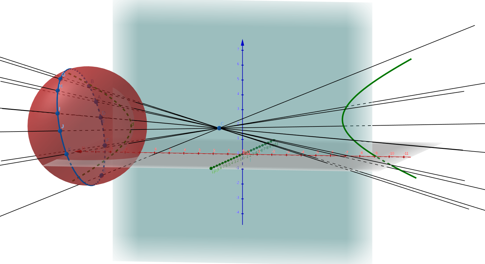
XIV. If a camera has square pixels, then the apparent contour of a sphere centred on the principal axis is a circle. If the sphere is translated parallel to the image plane, then the apparent contour deforms from a circle to an ellipse with the principal point on its major axis.
(a) How can this observation be used as a method of internal parameter calibration?
(b) Show by a geometric argument that the aspect ratio of the ellipse does not depend on the distance of the sphere from the camera.
If the sphere is now translated parallel to the principal axis the apparent contour can deform to a hyperbola, but only one branch of the hyperbola is imaged. Why is this?

(a) From the given information, we can conclude that when the camera has square pixels, the principal point will lie on the intersection of the major axes of the conic images of the two spheres. Hence, if we take the image of two spheres, we can obtain the principal point which is one of the internal parameters we are trying to determine.

(b) If the aspect ratio of the ellipse depended on the distance of the sphere from the camera centre then the aspect ratio must be the same for spheres equidistant from the centre. But that is clearly not the case as the image of the sphere is a circle when the sphere is centred on the principal axis and an ellipse otherwise. Similarly the aspect ratio of the ellipse should change with distance. This is not true for a sphere that is moved in the direction parallel to the line joining the camera centre and the sphere centre. Hence, the aspect ratio of the ellipse does not depend on the distance of the sphere from the camera.

(c) A hyperbola is formed when both halves of the cone of rays are intersected by the image plane. However, this is possible only when the sphere itself intersects the image plane. Hence, no image is recorded in that region and only the other half of the hyperbola is imaged. I think the question meant the sphere is translated perpendicular (not parallel) to the principal axis.

XV. Show that for a general camera the apparent contour of a sphere is related to the IAC as:$$\omega = C + \textbf{v}\textbf{v}^T$$ where $C$ is the conic outline of the imaged sphere, and $\textbf{v}$ is a 3-vector that depends on the position of the sphere. A proof is given in [Agrawal-03]. Note this relation places two constraints on $\omega$, so that in principle $\omega$, and hence the calibration $K$, may be computed from three images of a sphere. However, in practice this is not a well-conditioned method for computing $K$ because the deviation of the sphere’s outline from a circle is small.

The details are given in [Agrawal-03]⁴. Basically, we substitute the equation of the dual quadric $Q^*$ representing a sphere into the relation $PQ^*P^T$ where $P$ is the camera matrix to get the apparent contour $C$ of the sphere. We can derive the given relation by expressing $P$ in terms of $K$, $R$ and $t$.

References

comments powered by Disqus