Multiple View Geometry in Computer Vision Chapter 9 Solutions -- Epipolar Geometry and the Fundamental Matrix

Here’s a quick index to all the problems in this chapter.

The main index can be found here.

I. Fixating cameras. Suppose two cameras fixate on a point in space such that their principal axes intersect at that point. Show that if the image coordinates are normalized so that the coordinate origin coincides with the principal point then the $F_{33}$ element of the fundamental matrix is zero.

We know that two corresponding points $x$ and $x’$ must obey the relationship $x’^TFx = 0$. In this case it is given that $x = x’ = (0, 0, 1)^T$. Hence the constraint on $F$ becomes $$\begin{pmatrix}0 & 0 & 1 \end{pmatrix} F \begin{pmatrix}0 \\ 0 \\ 1 \end{pmatrix}= 0$$ which implies that $F_{33} = 0$.

II. Mirror images. Suppose that a camera views an object and its reflection in a plane mirror. Show that this situation is equivalent to two views of the object, and that the fundamental matrix is skew-symmetric. Compare the fundamental matrix for this configuration with that of: (a) a pure translation, and (b) a pure planar motion. Show that the fundamental matrix is auto-epipolar (as is (a)).

Let a point on the object be $\mathtt{X}$. Then a point on the reflection will be $\mathtt{R_fX}$, where $\mathtt{R_f}$ represents the 3D reflection. Under the camera $\mathtt{P}$ the images of the two points will be $\mathtt{PX}$ and $\mathtt{PR_fX}$. This situation is equivalent to two cameras $P$ and $\mathtt{PR_f}$ both viewing $\mathtt{X}$.

A reflection $\mathtt{R_f}$ about an arbitrary plane can be decomposed as $\mathtt{R_f = H_e \begin{pmatrix}\Lambda & \bf{0} \\ \bf{0}^T & 1\end{pmatrix}H_e^{-1}}$, where $\mathtt{H_e}$ is a Euclidean transformation $\mathtt{\begin{pmatrix}R & \bf{t} \\ \bf{0} & 1 \end{pmatrix}}$ and $\mathtt{\Lambda} = diag(-1, 1, 1)$. The proof of this statement is given at the end of this solution.

Without loss of generality, we can take $\mathtt{P = K[I \mid \bf{0}]}$. Then the second camera will be $\mathtt{PR_f = K[I \mid \bf{0}]}\mathtt{H_e\Lambda H_e^{-1}}$. We can write this in terms of $\mathtt{R}$ and $\mathtt{t}$ as $\mathtt{PR_f = K[R\Lambda R^T \mid -R\Lambda R^Tt + t]} = \mathtt{K[R\Lambda R^T \mid R\Gamma R^Tt]}$, where $\mathtt{\Gamma = I - \Lambda} = \begin{pmatrix} 2 & 0 & 0 \\ 0 & 0 & 0 \\ 0 & 0 & 0 \end{pmatrix}$.

The corresponding canonical cameras¹ will be $\mathtt{[I \mid \bf{0}]}$ and $\mathtt{K[R\Lambda R^TK^{-1} \mid R\Gamma R^Tt]}$ and from Result 9.9 (pg 254), the fundamental matrix relating these two cameras will be $\mathtt{F = [K R\Gamma R^Tt]_{\times}}\mathtt{KR\Lambda R^TK^{-1}}$.

To check if this matrix is skew-symmetric, we must check if it satisfies $\mathtt{x^TFx = 0}$ for all $\mathtt{x}$. $$\mathtt{x^TFx = x^T[K R\Gamma R^Tt]_{\times}}\mathtt{KR\Lambda R^TK^{-1}x}$$

Using result A4.3(p582), we get $$\mathtt{x^TFx = x^TK^{-T}[R\Gamma R^Tt]_{\times}}\mathtt{R\Lambda R^TK^{-1}x}$$ $$\mathtt{= (K^{-1}x)^T[R\Gamma R^Tt]_{\times}}\mathtt{R\Lambda R^T(K^{-1}x)}$$

Replacing $\mathtt{K^{-1}x}$ by $\mathtt{x’}$, we can rewrite this as $$\mathtt{x’^T[R\Gamma R^Tt]_{\times}}\mathtt{R\Lambda R^Tx’}$$

So now we just have to check if $\mathtt{[R\Gamma R^Tt]_{\times}}\mathtt{R\Lambda R^T}$ is skew symmetric. Using result A4.3(p582) again, we get $$\mathtt{R[\Gamma R^Tt]_{\times}}\mathtt{\Lambda R^T}$$ This matrix is skew symmetric as $\mathtt{[\Gamma R^Tt]_{\times}}$ is a matrix of the form $$\begin{pmatrix} 0 & 0 & 0 \\ 0 & 0 & -x \\ 0 & x & 0 \end{pmatrix}$$

This also means $F$ is auto-epipolar.

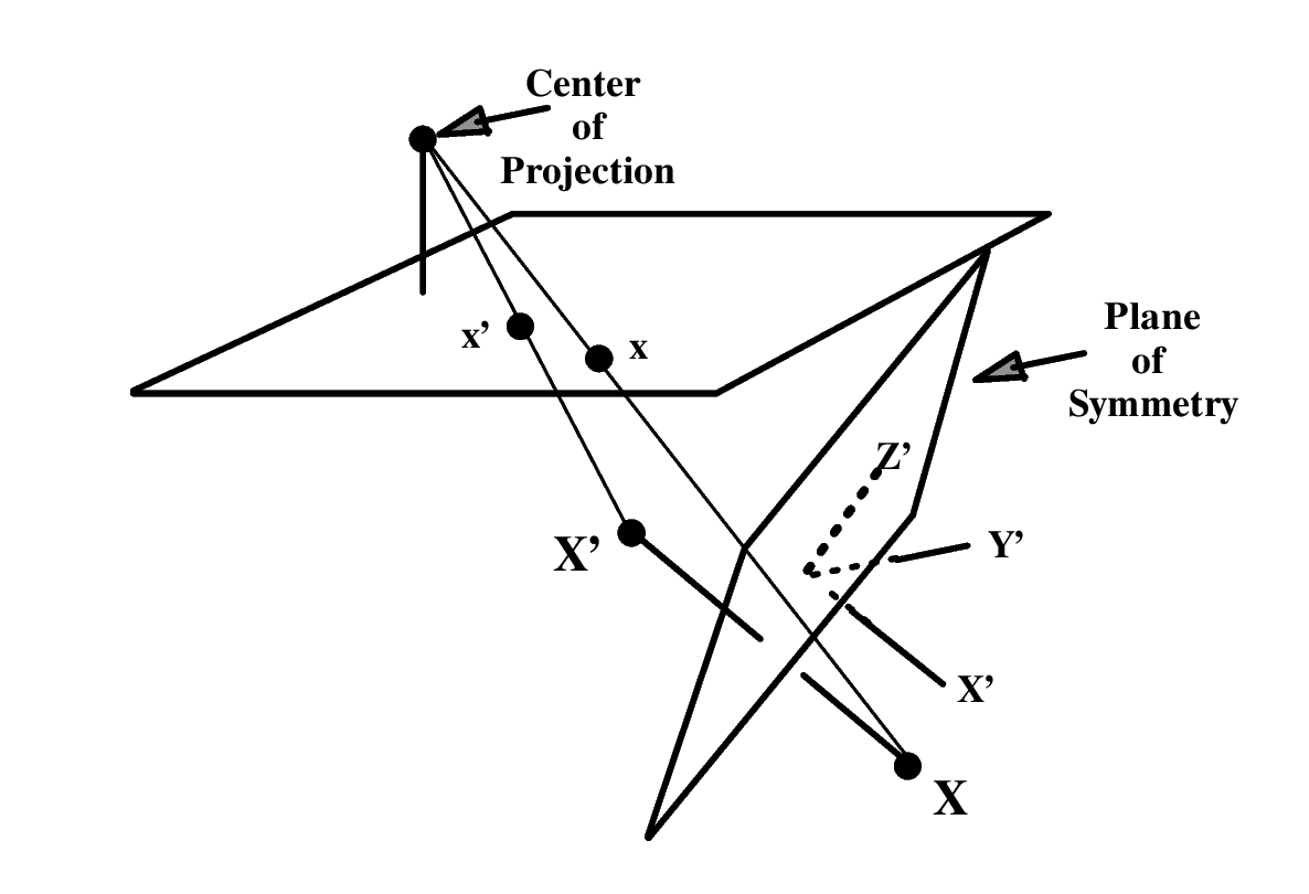
Just like in the case of translation where the epipole was the vanishing point of the direction of translation, in this case, the epipole is the vanishing point of the direction of reflection i.e. the normal to the plane of reflection or the direction of the symmetry line joining a point and its reflection ($\mathtt{X}$ and $\mathtt{X’}$ in the figure below).

The coordinate system for bilateral symmetry

Joseph L. Mundy and Andrew Zisserman. Repeated structures: Image correspondence constraints and 3D structure recovery.

Proof of $\mathtt{R_f = H_e \Lambda H_e^{-1}}$

A reflection $R_f$ about an arbitrary plane can be decomposed as a translation of the origin to the plane followed by a reflection followed by a translation of the origin back to the original position $R_f = TR_oT^{-1}$.

$R_o$ has the form $$R_o = \begin{pmatrix}A & \textbf{0} \\ \textbf{0}^T & 1 \end{pmatrix}$$ with the $3 \times 3$ matrix $A$ being a householder matrix. $A$ can be further decomposed using spectral decomposition to give $A = R\Lambda R^T$ with $\Lambda = diag(-1, 1, 1)$ and $R$ an orthogonal matrix.

So we can rewrite $R_f$ as

$$\mathtt{R_f = T\begin{pmatrix}R & \textbf{0} \\ \textbf{0}^T & 1 \end{pmatrix}\begin{pmatrix}\Lambda & \bf{0} \\ \bf{0}^T & 1\end{pmatrix} \begin{pmatrix}R^T & \textbf{0} \\ \textbf{0}^T & 1 \end{pmatrix}T^{-1}}$$

$$\implies \mathtt{R_f = \begin{pmatrix}I & \textbf{t}\end{pmatrix} \begin{pmatrix}R & \textbf{0} \\ \textbf{0}^T & 1 \end{pmatrix} \begin{pmatrix}\Lambda & \bf{0} \\ \bf{0}^T & 1\end{pmatrix} \begin{pmatrix}R & \textbf{0} \\ \textbf{0}^T & 1 \end{pmatrix}^{-1} \begin{pmatrix}I & \textbf{t}\end{pmatrix}^{-1}}$$

$$\implies \mathtt{R_f = \begin{pmatrix}R & \textbf{t} \\ \textbf{0}^T & 1 \end{pmatrix} \begin{pmatrix}\Lambda & \bf{0} \\ \bf{0}^T & 1\end{pmatrix} \begin{pmatrix}R & \textbf{t} \\ \textbf{0}^T & 1 \end{pmatrix}^{-1}}$$

$$\implies \mathtt{R_f = H_e \Lambda’ H_e^{-1}}$$

where $H_e$ represents the euclidean transformation given by $\begin{pmatrix}R & \textbf{t} \\ \textbf{0}^T & 1 \end{pmatrix}$ and $\mathtt{\Lambda’} = diag(-1, 1, 1, 1)$.

III. Show that if the vanishing line of a plane contains the epipole then the plane is parallel to the baseline.

The epipole is the vanishing point of the baseline direction. Parallel planes in 3-space intersect $\Pi_\infty$ in a common line and the image of this line is the vanishing line of the plane. So if the vanishing point of the baseline lies on this vanishing line then the baseline must lie in a plane parallel to the given plane.

IV. Show that the polar of $\textbf{x}_a$ intersects the Steiner conic $F_s$ at the epipoles (figure 9.10a). Hint, start from $F\textbf{e} = F_s\textbf{e} + F_a\textbf{e} = 0$. Since $\textbf{e}$ lies on the conic $F_s$, then $\textbf{l}_1 = F_s\textbf{e}$ is the tangent line at $\textbf{e}$, and $\textbf{l}_2 = F_a\textbf{e} = [x_\textbf{a}]_{\times}\textbf{e} = x_\textbf{a} \times \textbf{e}$ is a line through $\textbf{x}_a$ and $\textbf{e}$.

$$\mathtt{F\textbf{e} = F_s\textbf{e} + F_a\textbf{e} = 0}$$ $$\mathtt{\implies F_s\textbf{e} = -F_a\textbf{e}}$$

This means $\mathtt{F_s\textbf{e}}$ and $\mathtt{F_a\textbf{e}}$ are the same lines further implying that that the line through $\mathtt{\textbf{x}_a}$ and $\mathtt{\textbf{e}}$ is tangent to $\mathtt{F_s}$ at $\mathtt{\textbf{e}}$. Applying a similar logic to $\mathtt{\textbf{e}’ }$, it is clear that the lines through $\mathtt{\textbf{x}_a}$ tangent to $\mathtt{F_s}$ intersect $\mathtt{F_s}$ at $\mathtt{\textbf{e}}$ and $\mathtt{\textbf{e}’ }$. Hence $\mathtt{\textbf{e}}$ and $\mathtt{\textbf{e}’ }$ lie on the polar of $\mathtt{\textbf{x}_a}$.

VI. Planar motion. It is shown by [Maybank-93] that if the rotation axis direction is orthogonal or parallel to the translation direction then the symmetric part of the essential matrix has rank 2. We assume here that $K = K’$. Then from (9.12), $F = K^{-T}EK^{-1}$, and so $$F_s = (F + F^T)/2 = K^{-T}(E + E^T)K^{-1}/2 = K^{-T}E_sK^{-1}$$ It follows from $det(F_s) = det(K^{-1})^2det(E_s)$ that the symmetric part of $F$ is also singular. Does this result hold if $K \ne K’$?

If $\mathtt{K \ne K}$, then the equation becomes $$\mathtt{F_s = (F + F^T)/2 = K^{-T}EK’^{-1} + K’^{-T}E^TK^{-1}}$$

This equation can not be further reduced to a simpler form due to asymmetric components and hence we can not say anything about the rank of $\mathtt{F_s}$.

I think this question is incorrectly placed in this chapter as we haven’t really learnt about reconstructions yet. I might get back to this one after learning more about reconstruction in subsequent chapters.

IX. Following a similar development to section 9.2.2, derive the form of the fundamental matrix for two linear pushbroom cameras. Details of this matrix are given in [Gupta-97] where it is shown that affine reconstruction is possible from a pair of images.

As I’m not interested in pushbroom cameras at the moment, I’m going to skip this one.

References

Mundy, Joseph L., and Andrew Zisserman. Repeated structures: Image correspondence constraints and 3D structure recovery. Joint European-US Workshop on Applications of Invariance in Computer Vision. Springer, Berlin, Heidelberg, 1993. ^[return]