Introduction to Projective Geometry Solutions 5.6 -- Collineations of types II and III

Please read this introduction first before looking through the solutions. Here’s a quick index to all the problems in this section.

1 2 3 4 5 6 7 8 9 10

1. Show that no collineations of type II can be periodic.

The matrix in standard form for collineations of type II is as follows.

$⎛ ⎜ ⎝ \begin{matrix} k_{2} & a_{12} & 0 0 & k_{2} & 0 0 & 0 & k_{1} \end{matrix} ⎞ ⎟ ⎠$

Raising this to the $n^{t h}$ power we get

$⎛ ⎜ ⎜ ⎝ \begin{matrix} k_{2}^{n} & n a_{12} k_{2}^{n - 1} & 0 0 & k_{2}^{n} & 0 0 & 0 & k_{1}^{n} \end{matrix} ⎞ ⎟ ⎟ ⎠$

As $a_{12} \neq 0$ for $A - k_{2} I$ to be of rank 2 and $k_{2} \neq 0$ as a collineation is nonsingular by definition, the $n^{t h}$ power of a collineation of type II can never be a scalar multiple of $I$ . Hence a collineation of type II can not be periodic.

2. Under what conditions if any, can a collineation of type III be of period 2? Of period 3? Of period 4? Of period n?

The matrix in standard form for collineations of type III is as follows.

$⎛ ⎜ ⎝ \begin{matrix} k_{2} & 0 & 0 0 & k_{2} & 0 0 & 0 & k_{1} \end{matrix} ⎞ ⎟ ⎠$

Raising this to the $n^{t h}$ power we get

$⎛ ⎜ ⎜ ⎝ \begin{matrix} k_{2}^{n} & 0 & 0 0 & k_{2}^{n} & 0 0 & 0 & k_{1}^{n} \end{matrix} ⎞ ⎟ ⎟ ⎠$

For it to be of period $n$ , it must be a scalar multiple of $I$ . It is no specialization to take the scalar to be 1. So, for the $n^{t h}$ power of a collineation of type III to be of period $n$ , $k_{1}$ and $k_{2}$ must be distinct $p^{t h}$ roots of 1 such that $p \leq n$ and at least one of them is an $n^{t h}$ root of 1.

3. Show that the plane perspective transformation described in Chap. 1 is a collineation of type III.

This exercise ties things nicely together.

For a transformation to be a collineation of type III it must be nonsingular and it must have one point-by-point invariant line (corresponding to the repeated characteristic root) accompanied by an invariant point not on the invariant line (corresponding to the simple root).

Both these characteristics are displayed by the transformations described in Chap. 1. In $Π_{2}$ , each point has an image and each image has a pre-image proving that the transformation is nonsingular. The axis of transformation is the point-by-point invariant line and the center of transformation is the other invariant point not on the axis.

In fact if you look at the equations of transformation derived in the solution to exercise 1.2.16, we can express them in matrix form in homogeneous coordinates as follows

$⎛ ⎜ ⎝ \begin{matrix} - b & a & 0 0 & c & 0 0 & 1 & - b \end{matrix} ⎞ ⎟ ⎠$

This has characteristic roots $(c, - b)$ with multiplicity $(1, 2)$ respectively. The invariant point is $(a, b + c, 1)$ and the axis is given by the line, $x_{2} = 0$ , formed by the characteristic vectors, $(1, 0, 0), (0, 0, 1)$ , corresponding to the root $- b$ .

This matches with the $x$ -axis being the axis of transformation and the invariant point being $O$ after rabbatement.

4. If $P$ is a point on the line $F_{1} F_{2}$ , and if $P^{'}$ is its image under a collineation of type II, what is $℞ (F_{1} F_{2}, P P^{'})$ .

If the triangle of reference is defined such that $F_{1} : (0, 0, 1)$ and $F_{2} : (1, 0, 0)$ , any point on the line $F_{1} F_{2}$ will have $0$ as the value of the second coordinate.

Let’s denote the coordinates of a general point $P$ on $F_{1} F_{2}$ by $(p_{1}, 0, p_{3})$ . Its image under a collineation of type II represented by the matrix in #1 will be $(k_{2} p_{1}, 0, k_{1} p_{3})$ .

If the line $F_{1} F_{2}$ is parameterized by the points $F_{1}$ and $F_{2}$ , the coordinates of $P$ and its image $P^{'}$ will be $(p_{1}, p_{3})$ and $(k_{2} p_{1}, k_{1} p_{3})$ . Then the cross ratio of $(℞ F_{1} F_{2}, P P^{'})$ will be

$\frac{∣ ∣ ∣ \begin{matrix} 1 & 0 p_{1} & p_{3} \end{matrix} ∣ ∣ ∣ ∣ ∣ ∣ \begin{matrix} 0 & 1 k_{2} p_{1} & k_{1} p_{3} \end{matrix} ∣ ∣ ∣}{∣ ∣ ∣ \begin{matrix} 1 & 0 k_{2} p_{1} & k_{1} p_{3} \end{matrix} ∣ ∣ ∣ ∣ ∣ ∣ \begin{matrix} 0 & 1 p_{1} & p_{3} \end{matrix} ∣ ∣ ∣}$

$= \frac{p_{3} (- k_{2} p_{1})}{k_{1} p_{3} (- p_{1})}$

As $p_{1} \neq 0$ and $p_{3} \neq 0$ (else $P$ would be $F_{2}$ or $F_{1}$ )

$℞ (F_{1} F_{2}, P P^{'}) = \frac{k_{2}}{k_{1}}$

5. Find the fixed points of the transformation $X^{'} = A X$ if:

(a) $A = ⎛ ⎜ ⎝ \begin{matrix} 3 & 1 & - 1 - 6 & - 2 & 3 - 4 & - 2 & 3 \end{matrix} ⎞ ⎟ ⎠$ (b) $A = ⎛ ⎜ ⎝ \begin{matrix} - 4 & 3 & - 3 - 4 & 4 & - 5 2 & - 1 & 0 \end{matrix} ⎞ ⎟ ⎠$

(c) $A = ⎛ ⎜ ⎝ \begin{matrix} 9 & 3 & - 7 4 & 1 & - 2 12 & 4 & - 9 \end{matrix} ⎞ ⎟ ⎠$ (d) $A = ⎛ ⎜ ⎝ \begin{matrix} - 3 & - 2 & 2 12 & 7 & - 6 8 & 4 & - 3 \end{matrix} ⎞ ⎟ ⎠$

This one is pretty straightforward and you can use any software to find the eigenvectors of the given matrices. If the an eigenvalue is repeated then all the points on the line formed by the corresponding eigenvectors will be invariant. For a simple root only the eigenvector corresponding to it is invariant.

6. What is the locus of a point with the property that it and its image under a collineation of type II are collinear with a given point $O$ ? What is the locus of the images of such points?

Consider a general point $P : (p_{1}, p_{2}, p_{3})$ and its image $P^{'} : (p_{1}^{'}, p_{2}^{'}, p_{3}^{'})$ .

Using the equations of transformation of a general collineation of type II, we get

$p_{1}^{'} = k_{2} p_{1} + a_{12} p_{2}, p_{1} = \frac{p_{1}^{'} k_{2} - a_{12} p_{2}^{'}}{k_{2}^{2}}$ $p_{2}^{'} = k_{2} p_{2}, p_{2} = \frac{p_{2}^{'}}{k_{2}}$ $p_{3}^{'} = k_{1} p_{3}, p_{3} = \frac{p_{3}^{'}}{k_{1}}$

As per Sec 4.2, Theorem 1 if $P$ and its image are to be collinear with a given point $O : (o_{1}, o_{2}, o_{3})$ , we get

$∣ ∣ ∣ ∣ \begin{matrix} p_{1} & p_{2} & p_{3} k_{2} p_{1} + a_{12} p_{2} & k_{2} p_{2} & k_{1} p_{3} o_{1} & o_{2} & o_{3} \end{matrix} ∣ ∣ ∣ ∣ = 0$

Expanding this we get $(a_{12} o_{2} - k_{2} o_{1} + k_{1} o_{1}) p_{2} p_{3} + (k_{2} - k_{1}) o_{2} p_{1} p_{3} - a_{12} o_{3} p_{2}^{2} = 0$

Similarly, expressing in terms of image coordinates, we get

$∣ ∣ ∣ ∣ ∣ ∣ \begin{matrix} \frac{p_{1}^{'} k_{2} - a_{12} p_{2}^{'}}{k_{2}^{2}} & \frac{p_{2}^{'}}{k_{2}} & \frac{p_{3}^{'}}{k_{1}} p_{1}^{'} & p_{2}^{'} & p_{3}^{'} o_{1} & o_{2} & o_{3} \end{matrix} ∣ ∣ ∣ ∣ ∣ ∣ = 0$

Expanding this we get $(a_{12} o_{2} k_{1} + o_{1} k_{2} k_{1} - o_{1} k_{2}^{2}) p_{2} p_{3} + (k_{2} - k_{1}) o_{2} k_{2} p_{1} p_{3} - a_{12} o_{3} k_{1} p_{2}^{2} = 0$

In both cases the locus is a conic.

7. What are the equations of a collineation of type II with characteristic values $k_{1}$ , $k_{2}$ , $k_{2}$ if:
(a) The corresponding fixed points are $F_{1} : (0, 1, 0)$ and $F_{2} : (1, 1, 0)$ , and the second fixed line is $f_{2} : x_{1} - x_{2} = 0$ ?
(b) The corresponding fixed points are $F_{1} : (1, 0, 0)$ and $F_{2} : (0, - 1, 1)$ , and the second fixed line is $f_{2} : x_{1} = 0$ ?

Note: The answers for (a) and (b) are flipped in the book.

(a) As the second invariant line goes through $F_{2}$ it must be the characteristic vector associated with the repeated characteristic root $k_{2}$ .

As $F_{1}$ and $F_{2}$ are invariant points, under the transformation, $(0, 1, 0) \to (0, k_{1}, 0)$ and $(1, 1, 0) \to (k_{2}, k_{2}, 0)$ . Using this information in the equations of the general collineation, we get

$a_{12} = a_{32} = 0, a_{22} = k_{1}$ $a_{11} = k_{2}, a_{21} = k_{2} - k_{1}, a_{31} = 0$

Hence the equations of the transformation can be written as $x_{1}^{'} = k_{2} x_{1} + a_{13} x_{3}$ $x_{2}^{'} = (k_{2} - k_{1}) x_{1} + k_{1} x_{2} + a_{23} x_{3}$ $x_{3}^{'} = a_{33} x_{3}$

In matrix form this would be $A = ⎛ ⎜ ⎝ \begin{matrix} k_{2} & 0 & a_{13} k_{2} - k_{1} & k_{1} & a_{23} 0 & 0 & a_{33} \end{matrix} ⎞ ⎟ ⎠$

As $k_{2}$ must be a repeated root of $A - k I$ , $a_{33}$ must be $k_{2}$ .

As $f_{2}$ is the second fixed line, any point of the form $(1, 1, a)$ must be transformed to a point of the form $(1, 1, b)$ . Using this in the equations of transformation we get

$k_{2} + a_{13} a = 1$ $k_{2} + a_{23} a = 1$ $k_{2} a = b$

Hence, $a_{13} = a_{23}$ . Also, $a_{13} \neq 0$ as the rank of $A - k_{2} I$ must be 2. So the equations of transformation will be

$x_{1}^{'} = k_{2} x_{1} + a_{13} x_{3}$ $x_{2}^{'} = (k_{2} - k_{1}) x_{1} + k_{1} x_{2} + a_{13} x_{3}$ $x_{3}^{'} = k_{2} x_{3}$

(b) As the second invariant line goes through $F_{2}$ it must be the characteristic vector associated with the repeated characteristic root $k_{2}$ .

As $F_{1}$ and $F_{2}$ are invariant points, under the transformation, $(1, 0, 0) \to (k_{1}, 0, 0)$ and $(0, - 1, 1) \to (0, - k_{2}, k_{2})$ . Using this information in the equations of the general collineation, we get

$a_{21} = a_{31} = 0, a_{11} = k_{1}$ $a_{12} = a_{13}$ $a_{23} = a_{22} - k_{2}$ $a_{32} = a_{33} - k_{2}$

As $f_{2}$ is the second invariant line, a point of the form $(0, a, b)$ must have an image of the form $(0, c, d)$ . This implies that $a_{12} = 0$ .

Putting this all together, we get the matrix of transformation as follows.

$A = ⎛ ⎜ ⎝ \begin{matrix} k_{1} & 0 & 0 0 & a_{22} & a_{22} - k_{2} 0 & a_{33} - k_{2} & a_{33} \end{matrix} ⎞ ⎟ ⎠$

The characteristic equation of this matrix will be

$(k_{1} - k) ((a_{22} - k) (a_{33} - k) - (a_{22} - k_{2}) (a_{33} - k_{2})) = 0$

As this is a collineation of type II, the two quadratic roots of the second term must be equal to the repeated root of the collineation, $k_{2}$ . This means

$a_{33} + a_{22} - k_{2} = k_{2}$ $⟹ a_{33} = 2 k_{2} - a_{22}$

Hence the equations of transformation will be $x_{1}^{'} = k_{1} x_{1}$ $x_{2}^{'} = a_{22} x_{2} + (a_{22} - k_{2}) x_{3}$ $x_{3}^{'} = (k_{2} - a_{22}) x_{2} + (2 k_{2} - a_{22}) x_{3}$ 7 As the rank of $A - k_{2} I$ must be 2, $a_{22} \neq k_{2}$ .

8. (a) Show that any collineation of type I can be obtained as the composition of two collineations of type III.
(b) Can every collineation of type III be obtained as the composition of two collineations of type II?

(a) Consider two collineations $A$ and $B$ of type III with characteristic roots $a_{1}$ , $a_{2}$ , $a_{2}$ and $b_{1}$ , $b_{2}$ , $b_{2}$ , centers $F_{A}$ , $F_{B}$ and axes $f_{a}$ and $f_{b}$ respectively such that $F_{B}$ lies on $f_{a}$ and $F_{A}$ lies on $f_{b}$ . Let the intersection of $f_{a}$ and $f_{b}$ be $F_{A B}$ . So we get

$A B F_{A} = A (b_{2} F_{A}) = b_{2} A F_{A} = b_{2} a_{1} F_{A}$ $A B F_{B} = A (b_{1} F_{B}) = b_{1} A F_{B} = b_{1} a_{2} F_{B}$ $A B F_{A B} = A (b_{2} F_{A B}) = b_{2} A F_{A B} = b_{2} a_{2} F_{A B}$

Hence the collineation $A B$ is a collineation of type I with characteristic roots $a_{1} b_{2}$ , $a_{2} b_{1}$ and $a_{2} b_{2}$ and corresponding fixed points $F_{A}$ , $F_{B}$ and $F_{A B}$ respectively.

Now if we represent the three roots as $k_{1}$ , $k_{2}$ and $k_{3}$ , we will get

$k_{1} = a_{1} b_{2}$ $k_{2} = a_{2} b_{1}$ $k_{3} = a_{2} b_{2}$

For any given $k_{1}$ , $k_{2}$ and $k_{3}$ the values $a_{1} = \frac{k_{1}}{k_{3}}$ , $a_{2} = 1$ , $b_{1} = k_{2}$ and $b_{2} = k_{3}$ satisfy these constraints.

Hence any collineation of type I with characteristic roots $k_{1}$ , $k_{2}$ and $k_{3}$ and corresponding fixed points $F_{1}$ , $F_{2}$ and $F_{3}$ can be represented as the composition of the following two collineations of type III.

Center $F_{1}$ and axis $F_{2} F_{3}$ with characteristic roots $\frac{k_{1}}{k_{3}}$ , 1 and 1.
Center $F_{2}$ and axis $F_{1} F_{3}$ with characteristic roots $k_{2}$ , $k_{3}$ , and $k_{3}$ .

To verify this, let’s multiply the matrices of the collineations of type III to see if we get back the collineation of type I.

Assuming the coordinate system to be specialized so that $F_{1}$ , $F_{2}$ and $F_{3}$ are the vertices of the triangle of reference, the matrices of transformation for the collineations of type III will be

$A = ⎛ ⎜ ⎜ ⎝ \begin{matrix} \frac{k_{1}}{k_{3}} & 0 & 0 0 & 1 & 0 0 & 0 & 1 \end{matrix} ⎞ ⎟ ⎟ ⎠$

$B = ⎛ ⎜ ⎝ \begin{matrix} k_{3} & 0 & 0 0 & k_{2} & 0 0 & 0 & k_{3} \end{matrix} ⎞ ⎟ ⎠$

And their composition $A B$ will be

$⎛ ⎜ ⎜ ⎝ \begin{matrix} \frac{k_{1}}{k_{3}} & 0 & 0 0 & 1 & 0 0 & 0 & 1 \end{matrix} ⎞ ⎟ ⎟ ⎠ ⎛ ⎜ ⎝ \begin{matrix} k_{3} & 0 & 0 0 & k_{2} & 0 0 & 0 & k_{3} \end{matrix} ⎞ ⎟ ⎠$ $= ⎛ ⎜ ⎝ \begin{matrix} k_{1} & 0 & 0 0 & k_{2} & 0 0 & 0 & k_{3} \end{matrix} ⎞ ⎟ ⎠$

which is the collineation of type I that we started out to decompose.

(b) I’ll be honest, this one threw me for a loop. I had to think about it for a couple of days and my brain calling me a dumb-dumb for not being able to solve a teeny-weeny part (b) of an even numbered problem didn’t make things any easier.

It all boils down to whether the collineations of type II can compose to preserve the invariant properties of a collineation of type III while fulfilling their own constraints.

We know that a collineation of type III has a point of fixed lines, the center, and a line of fixed points, the axis. So the composition of the collineations of type II must preserve these two properties.

A collineation of type II alone can’t preserve a point of fixed lines, by definition. So one of the two collineations of type II must be transforming each fixed line through the center to another line, and the other must be reversing this transformation to get back the original line. This means the point of intersection of the original invariant line and its image must be invariant under both the collineations of type II, and this must be true for each fixed line through the center. However, collineations of type II only have 2 fixed points. Thus no collineation of type III can be expressed as a composition of two collineations of type II.

9. If $T_{1}$ is the harmonic homology whose center is the point $C_{1} : (1, - 1, 0)$ and whose axis is the line $l : x_{1} - x_{2} = 0$ , and if $T_{2}$ is the quadratic inversion defined by the point $C_{2} : (0, 0, 1)$ and the conic $Γ : x_{3}^{2} - x_{1} x_{2} = 0$ , find the equations of $T_{1}$ and $T_{2}$ and show that $T_{1}$ and $T_{2}$ commute. Show also that $T = T_{1} T_{2}$ is of period 2.

Let $P : (p_{1}, p_{2}, p_{3})$ be a general point.

The equation of $P C_{1}$ is $(p_{1}, p_{2}, p_{3}) \times (1, - 1, 0) = [p_{3}, p_{3}, - p_{1} - p_{2}]$

The intersection of $P C_{1}$ with the axis is $C_{1}^{'} : [p_{3}, p_{3}, - p_{1} - p_{2}] \times [1, - 1, 0] = (- p_{1} - p_{2}, - p_{1} - p_{2}, - 2 p_{3})$

If the line $P C_{1}$ is parameterized by $C_{1}$ and $C_{1}^{'}$ , the parameters of $P$ will be $(p_{1} - p_{2}, - 1)$ . By Lemma 2 Section 4.7, the parameters of the harmonic conjugates of $P$ with respect to $C_{1}$ and $C_{1}^{'}$ will be $(p_{1} - p_{2}, 1)$ . Hence $P^{'}$ , the image of $P$ , under this harmonic homology is $(p_{2}, p_{1}, p_{3})$ and the equations of transformation for $T_{1}$ will be

$p_{1}^{'} = p_{2}$ $p_{2}^{'} = p_{1}$ $p_{3}^{'} = p_{3}$

As per Sec 3.7, the intersections $S$ and $T$ of $P C_{2}$ with $Γ$ will be the solution to the quadratic equation

$λ^{2} P^{T} A P + 2 λ μ P^{T} A C_{2} + μ^{2} C_{2}^{T} A C_{2} = 0$

where $A = ⎛ ⎜ ⎜ ⎝ \begin{matrix} 0 & - \frac{1}{2} & 0 - \frac{1}{2} & 0 & 0 0 & 0 & 1 \end{matrix} ⎞ ⎟ ⎟ ⎠$ .

Evaluating, we have $P^{T} A P = p_{3}^{2} - p_{1} p_{2}$ , $P^{T} A C_{2} = p_{3}$ and $C_{2}^{T} A C_{2} = 1$ . So the equation above becomes $λ^{2} (p_{3}^{2} - p_{1} p_{2}) + 2 λ μ p_{3} + μ^{2} = 0$ The parameters of intersection are thus $(- 1, p_{3} + \sqrt{p_{1} p_{2}})$ , $(- 1, p_{3} - \sqrt{p_{1} p_{2}})$ and the corresponding coordinates are $S : (- p_{1}, - p_{2}, \sqrt{p_{1} p_{2}})$ and $T : (p_{1}, p_{2}, \sqrt{p_{1} p_{2}})$ .

Taking $S$ and $T$ to be the parameters of the line $P C_{2}$ , the parameters of $P$ will be $(p_{3} - \sqrt{p_{1} p_{2}}, p_{3} + \sqrt{p_{1} p_{2}})$ . According to Lemma 2 Section 4.7, the parameters of $P^{'}$ the harmonic conjugate of $P$ with respect to $S$ and $T$ should be $(- p_{3} + \sqrt{p_{1} p_{2}}, p_{3} + \sqrt{p_{1} p_{2}})$ . Hence the coordinates of $P^{'}$ under this quadratic inversion will be $(p_{1} p_{3}, p_{2} p_{3}, p_{1} p_{2})$ and the equations of transformation for $T_{2}$ will be

$p_{1}^{'} = p_{1} p_{3}$ $p_{2}^{'} = p_{2} p_{3}$ $p_{3}^{'} = p_{1} p_{2}$

Clearly, the equations of transformation of $T_{1} T_{2}$ and $T_{2} T_{1}$ will be

$p_{1}^{'} = p_{2} p_{3}$ $p_{2}^{'} = p_{1} p_{3}$ $p_{3}^{'} = p_{1} p_{2}$

Hence $T_{1} T_{2} = T_{2} T_{1}$ .

Applying this transformation twice, the coordinates of the image will be $(p_{1}^{2} p_{2} p_{3}, p_{2}^{2} p_{1} p_{3}, p_{3}^{2} p_{1} p_{2})$ which is $(p_{1}, p_{2}, p_{3})$ . Hence $T_{1} T_{2}$ has a period of 2.

10. In Exercise 9, what is the image of each side of the triangle of reference under the transformation $T = T_{1} T_{2}$ ? What can be said about the curve into which $T$ transforms a conic which is tangent to each side of the triangle of reference? What can be said of the curve into which $T$ transforms a conic which intersects each side of the triangle of reference in two real points? What are the images under $T$ of the vertices of the triangle of reference? What is the image under $T$ of a conic which passes through the vertices of the triangle of reference?

This problem exposed me to the concepts of nonlinear transformations and algebraic curves¹. I always wondered what name to give curves that have two parameters $x$ and $y$ , now I know.

To find the images of the sides we first have to find the equations of the inverse of $T_{1} T_{2}$ . These are $p_{1}^{2} = \frac{p_{2}^{'} p_{3}^{'}}{p_{1}^{'}}$ $p_{2}^{2} = \frac{p_{1}^{'} p_{3}^{'}}{p_{2}^{'}}$ $p_{3}^{2} = \frac{p_{2}^{'} p_{1}^{'}}{p_{3}^{'}}$

The equations for the sides of the reference triangle are $p_{1} = 0$ $p_{2} = 0$ $p_{3} = 0$

Squaring these and using the equations of the inverse of $T$ we get $p_{2}^{'} p_{3}^{'} = 0$ $p_{1}^{'} p_{3}^{'} = 0$ $p_{2}^{'} p_{1}^{'} = 0$

So the equations of the sides of the reference triangle become singular conics $x_{2} x_{3} = 0$ , $x_{1} x_{3} = 0$ , $x_{2} x_{1} = 0$ under the nonlinear transformation $T_{1} T_{2}$ . Basically, a line gets transformed to two lines!

We know from Theorem 13, Section 4.9 that if a line $Λ$ is tangent to a conic with the matrix of quadratic form $A$ then $Λ^{T} A^{- 1} Λ = 0$ .

Applying this to the general matrix $A$ of a conic that is tangent to each side of the triangle of reference and representing its inverse by B, we get $b_{11} = b_{22} = b_{33} = 0$ . So $B$ looks like $B = ⎛ ⎜ ⎝ \begin{matrix} 0 & b_{12} & b_{13} b_{12} & 0 & b_{23} b_{13} & b_{23} & 0 \end{matrix} ⎞ ⎟ ⎠$ Inverting this, we get $B^{- 1} = A = ⎛ ⎜ ⎜ ⎝ \begin{matrix} - b_{23}^{2} & b_{13} b_{23} & b_{12} b_{23} b_{12} b_{23} & - b_{13}^{2} & b_{12} b_{13} b_{12} b_{23} & b_{12} b_{13} & - b_{12}^{2} \end{matrix} ⎞ ⎟ ⎟ ⎠$ So the equation of the conic will be $$b^2_{23}p^2_1 + b^2_{13}p^2_2 + b^2_{12}p^2_3 - 2b_{13}b_{23}p_1p_2

2b_{12}b_{23}p_1p_3 - 2b_{12}b_{13}p_2p_3 = 0$$

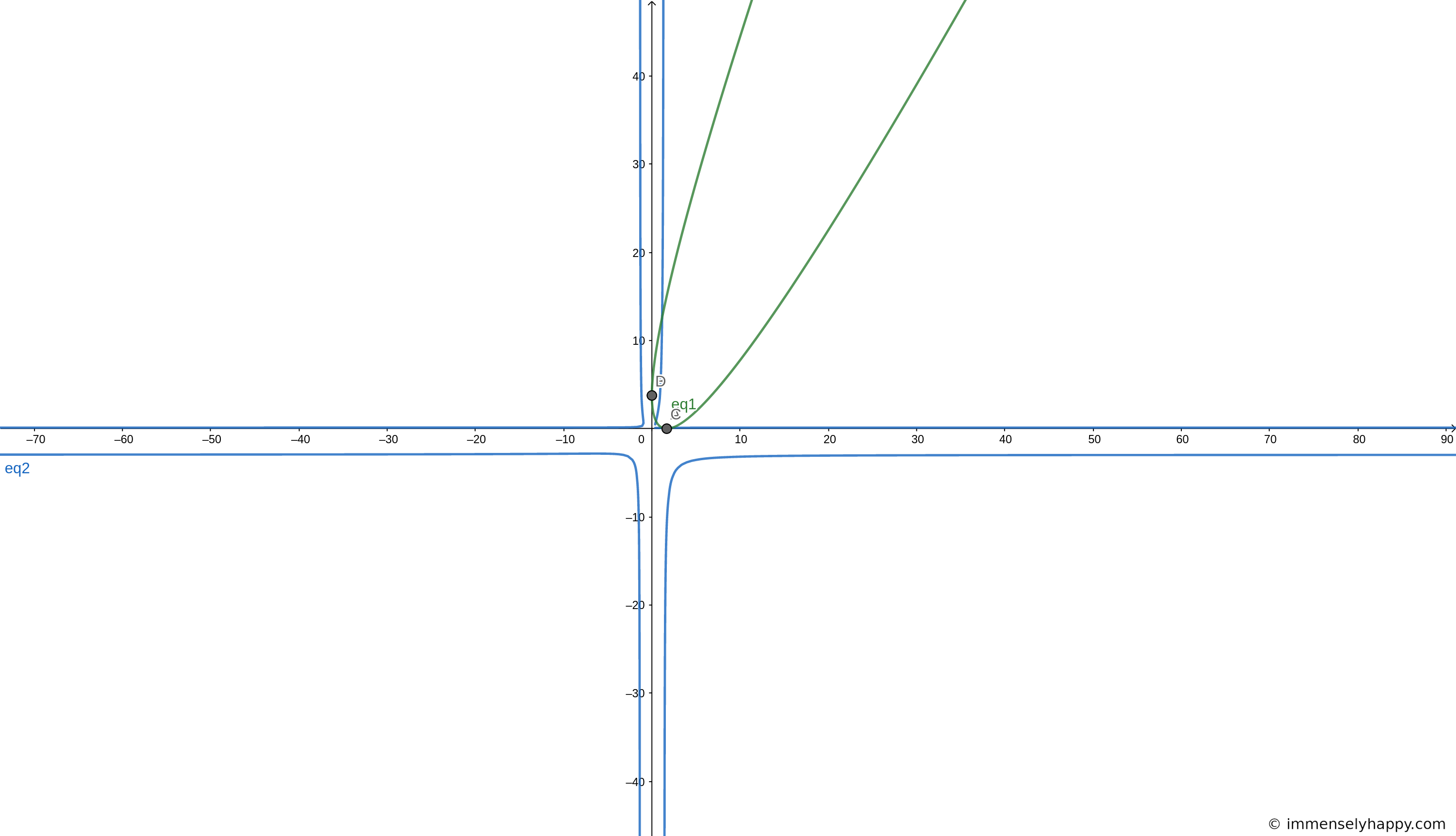
Using the equations of the inverse transform, we get $$b^2_{23}\frac{p'_2p'_3}{p'_1} + b^2_{13}\frac{p'_1p'_3}{p'_2} + b^2_{12}\frac{p'_2p'_1}{p'_3} - 2b_{13}b_{23}p'_3

2b_{12}b_{23}p'_2 - 2b_{12}b_{13}p'_1 = 0 $M u l t i p l y i n g b o t h s i d e s b y $ p_{1}^{'} p_{2}^{'} p_{3}^{'} $, w e g e t$ b^2_{23}(p'_2p'_3)^2 + b^2_{13}(p'_1p'_3)^2 + b^2_{12}(p'_2p'_1)^2 \\ - 2b_{13}b_{23}p'_1p'_2p'^2_3 - 2b_{12}b_{23}p'_1p'^2_2p'_3 - 2b_{12}b_{13}p'^2_1p'_2p'_3 = 0$$

This is a quartic curve². As you can see from the image below, it kind of looks like a cruciform curve³ but it’s not. Maybe someone who’s better at algebraic geometry than me can tell me if this type of curve has a special name.

View in GeoGebra

If a conic intersects each side of the reference triangle in 2 points then each of these quadratic equations must have 2 solutions. $a_{11} λ^{2} + 2 λ μ a_{12} + a_{22} μ^{2} = 0$ $a_{22} λ^{2} + 2 λ μ a_{23} + a_{33} μ^{2} = 0$ $a_{33} λ^{2} + 2 λ μ a_{13} + a_{11} μ^{2} = 0$ So, $a_{12}^{2} \neq a_{22} a_{11}$ $a_{23}^{2} \neq a_{22} a_{33}$ $a_{13}^{2} \neq a_{33} a_{11}$ Well that’s not much to go by so we can just represent such a conic with the general quadratic equation $a_{11} p_{1}^{2} + $ a_{22} p_{2}^{2} + a_{33} p_{3}^{2} + a_{12} p_{1} p_{2} + a_{13} p_{1} p_{3} + a_{23} p_{2} p_{3} = 0$ with its image under the given transformation being $a_{11} \frac{p_{2}^{'} p_{3}^{'}}{p_{1}^{'}} + a_{22} \frac{p_{1}^{'} p_{3}^{'}}{p_{2}^{'}} + a_{33} \frac{p_{1}^{'} p_{2}^{'}}{p_{3}^{'}} + a_{12} p_{3}^{'} + a_{13} p_{2}^{'} + a_{23} p_{1}^{'} = 0$ Multiplying by $p_{1}^{'} p_{2}^{'} p_{3}^{'}$ we get $a_{11} (p_{2}^{'} p_{3}^{'})^{2} + a_{22} (p_{1}^{'} p_{3}^{'})^{2} + a_{33} (p_{1}^{'} p_{2}^{'})^{2} + a_{12} p_{1}^{'} p_{2}^{'} p_{3}^{' 2} + a_{13} p_{1}^{'} p_{2}^{' 2} p_{3}^{'} + a_{23} p_{1}^{' 2} p_{2}^{'} p_{3}^{'} = 0$ which is the equation of a general quartic curve.

The vertices of the triangle of reference do not have images under this transformation.

The matrix of transformation of a conic that is contains the vertices of the triangle of reference will be $B$ as given above and its equation will be $b_{12} p_{1} p_{2} + b_{13} p_{1} p_{3} + b_{23} p_{2} p_{3} = 0$

Using the equations of transformation, the image of this conic will be $b_{12} p_{3}^{'} + b_{13} p_{2}^{'} + b_{23} p_{1}^{'} = 0$ which is the equation of a line. So under this transformation, a conic can get transformed into a line!

References

Wikipedia. Algebraic curves. https://en.wikipedia.org/wiki/Algebraic_curve. ↩︎
Wikipedia. Quartic plane curve. https://en.wikipedia.org/wiki/Quartic_plane_curve. ↩︎
Wolfram Mathworld. Cruciform curve. http://mathworld.wolfram.com/Cruciform.html. ↩︎

1. Show that no collineations of type II can be periodic.

2. Under what conditions if any, can a collineation of type III be of period 2? Of period 3? Of period 4? Of period n?

3. Show that the plane perspective transformation described in Chap. 1 is a collineation of type III.

4. If P is a point on the line F1F2, and if P′ is its image under a collineation of type II, what is ℞(F1F2,PP′).

5. Find the fixed points of the transformation X′=AX if:

6. What is the locus of a point with the property that it and its image under a collineation of type II are collinear with a given point O? What is the locus of the images of such points?

8. (a) Show that any collineation of type I can be obtained as the composition of two collineations of type III. (b) Can every collineation of type III be obtained as the composition of two collineations of type II?

References

4. If $P$ is a point on the line $F_{1} F_{2}$ , and if $P^{'}$ is its image under a collineation of type II, what is $℞ (F_{1} F_{2}, P P^{'})$ .

5. Find the fixed points of the transformation $X^{'} = A X$ if:

6. What is the locus of a point with the property that it and its image under a collineation of type II are collinear with a given point $O$ ? What is the locus of the images of such points?

8. (a) Show that any collineation of type I can be obtained as the composition of two collineations of type III.
(b) Can every collineation of type III be obtained as the composition of two collineations of type II?